04 vls
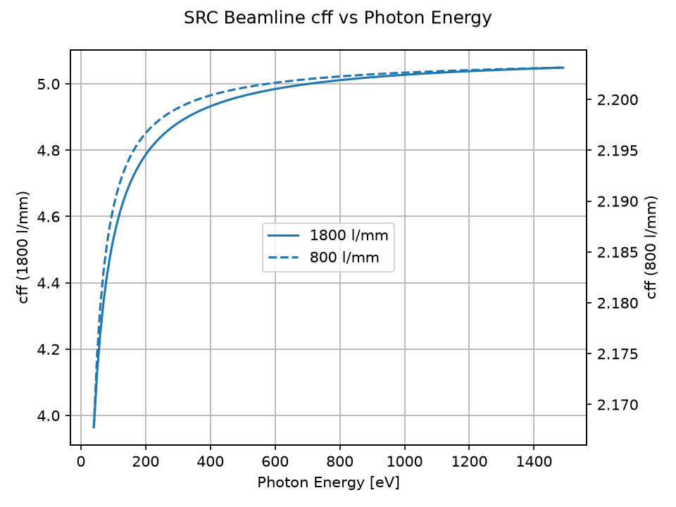
This example uses the variable-line-spacing helpers to compute and plot the cff dependence over photon energy.
import matplotlib.pyplot as plt
import numpy as np

from raypyng.vls_grating import calculate_vls_coeff
from raypyng.vls_grating import cff_for_fixed_focus
from raypyng.vls_grating import N1_to_b2

calculate_vls_coeff(alpha_g_deg=89.778, beta_g_deg=85.5733,
                        N0_lpm=2400,  # lines per mm
                        m=1, en_eV=1000,
                        source_vls_distance=81,
                        vls_image_distance=35,
                        verbose=True)


# Compute the CFF (c-value) required to keep the image (focus) position fixed
# when scanning photon energy with a plane VLS grating.
# This example reproduces the plot in the Reininger and de Castro paper
# for the SRC beamline, Figure 4.
# https://doi.org/10.1016/j.nima.2004.09.007

energies = np.arange(40, 1500, 10)

# 1800 l/mm
c_list_1800 = []
c_list_800 = []
n1_1800 = 37.443
n1_800 = 20.147
b2_1800 = N1_to_b2(n1_1800, k=1800)
b2_800 = N1_to_b2(n1_800, k=800)

for energy in energies:
    c_list_1800.append(cff_for_fixed_focus(
        B2=b2_1800,
        en_eV=energy,
        N0_lpmm=1800,
        source_vls_distance_m=27.2,
        vls_image_distance_m=10,
        r_override=0,
        verbose=False,
        ))

    c_list_800.append(cff_for_fixed_focus(
        B2=b2_800,
        en_eV=energy,
        N0_lpmm=800,
        source_vls_distance_m=27.2,
        vls_image_distance_m=10,
        r_override=0,
        verbose=False,
        ))

fig, ax1 = plt.subplots()

# Left y-axis: 1800 l/mm
ax1.plot(energies, c_list_1800,linestyle='solid', label='1800 l/mm')
ax1.set_xlabel('Photon Energy [eV]')
ax1.set_ylabel('cff (1800 l/mm)')
ax1.grid(True)

# Right y-axis: 800 l/mm
ax2 = ax1.twinx()
ax2.plot(energies, c_list_800, linestyle='dashed', label='800 l/mm')
ax2.set_ylabel('cff (800 l/mm)')

# Title
fig.suptitle('SRC Beamline cff vs Photon Energy')

# Combined legend (important)
lines1, labels1 = ax1.get_legend_handles_labels()
lines2, labels2 = ax2.get_legend_handles_labels()
ax1.legend(lines1 + lines2, labels1 + labels2, loc='center')

fig.tight_layout()
fig.savefig("vls_cff_vs_energy.png", dpi=150)
plt.close(fig)
Result: