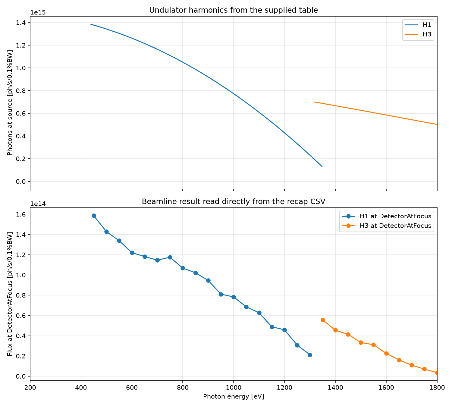
08 external undulator flux table

This example shows how to use an external undulator flux table. The top-level recap file DetectorAtFocus_RawRaysOutgoing.csv contains the geometric results together with the harmonic-resolved flux columns such as PhotonFlux1 and FluxPerMilPerBwAbs1. That recap file is the main result to inspect and plot after the simulation. Outside the tabulated energy window of a harmonic, the harmonic-derived recap columns are written as NaN so the plot can ignore them naturally.

The simulation script:

from raypyng import Simulate
import numpy as np
import os
import pandas as pd


if __name__ == '__main__':
    this_file_dir = os.path.dirname(os.path.realpath(__file__))
    rml_file = os.path.join(this_file_dir, '..', 'rml', 'simple_undulator_beamline.rml')

    sim = Simulate(rml_file, hide=True)
    sim.path = this_file_dir  # write output inside this example's own folder

    rml = sim.rml
    beamline = sim.rml.beamline

    # define the values of the parameters to scan
    energy = np.arange(200, 1800.1, 50)
    SlitSize = np.array([0.1])
    cff = np.array([2.25])
    nrays = 1e5

    params = [
        {beamline.SU.photonEnergy: energy},
        {beamline.ExitSlit.totalHeight: SlitSize},
        {beamline.PG.cFactor: cff},
        {beamline.SU.numberRays: nrays},
    ]

    sim.params = params
    sim.simulation_name = 'external_undulator_flux_table'
    sim.repeat = 4
    sim.analyze = False
    sim.raypyng_analysis = True

    sim.exports = [
        {beamline.SU: ['RawRaysOutgoing']},
        {beamline.DetectorAtFocus: ['RawRaysOutgoing']},
    ]

    undulator_file_path = os.path.join(
        this_file_dir, '..', 'undulator', 'undulator_harmonics_energy_photons.csv'
    )
    sim.undulator_table = pd.read_csv(undulator_file_path)

    sim.run(multiprocessing="auto", force=True)

The eval script:

import os

import matplotlib

matplotlib.use("Agg")

import matplotlib.pyplot as plt  # noqa: E402
import pandas as pd  # noqa: E402


if __name__ == "__main__":
    this_file_dir = os.path.dirname(os.path.realpath(__file__))

    undulator = pd.read_csv(
        os.path.join(
            this_file_dir,
            "..",
            "undulator",
            "undulator_harmonics_energy_photons.csv",
        )
    )
    detector = pd.read_csv(
        os.path.join(
            this_file_dir,
            "RAYPy_Simulation_external_undulator_flux_table",
            "DetectorAtFocus_RawRaysOutgoing.csv",
        )
    ).sort_values("PhotonEnergy")

    fig, axs = plt.subplots(2, 1, figsize=(10, 9), sharex=True)
    xmin = detector["PhotonEnergy"].min()
    xmax = detector["PhotonEnergy"].max()

    axs[0].plot(undulator["Energy1[eV]"], undulator["Photons1"], label="H1")
    axs[0].plot(undulator["Energy3[eV]"], undulator["Photons3"], label="H3")
    axs[0].set(
        ylabel="Photons at source [ph/s/0.1%BW]",
        title="Undulator harmonics from the supplied table",
    )
    axs[0].set_xlim(xmin, xmax)
    axs[0].grid(True, alpha=0.3)
    axs[0].legend()

    axs[1].plot(
        detector["PhotonEnergy"],
        detector["FluxPerMilPerBwAbs1"],
        marker="o",
        label="H1 at DetectorAtFocus",
    )
    axs[1].plot(
        detector["PhotonEnergy"],
        detector["FluxPerMilPerBwAbs3"],
        marker="o",
        label="H3 at DetectorAtFocus",
    )
    axs[1].set(
        xlabel="Photon energy [eV]",
        ylabel="Flux at DetectorAtFocus [ph/s/0.1%BW]",
        title="Beamline result read directly from the recap CSV",
    )
    axs[1].set_xlim(xmin, xmax)
    axs[1].grid(True, alpha=0.3)
    axs[1].legend()

    fig.tight_layout()
    out_png = os.path.join(this_file_dir, "eval_external_undulator_flux_table.png")
    fig.savefig(out_png, dpi=150)
    print("[eval] saved:", out_png)

Result: